TrackMate v7.7.0: New Hessian detector and new actions.
This new version focuses on bringing new feature to TrackMate.
Mainly:
- A new spot detector, based on the determinant of the Hessian (DoH), the Hessian detector.
- A new action that can measure the distance from spots to ROIs, possibly over time.
- A new option in the label exporter that allows setting the label IDs from the spot IDs.
A new spot detector based on the determinant of Hessian (DoH).
A. Principle.
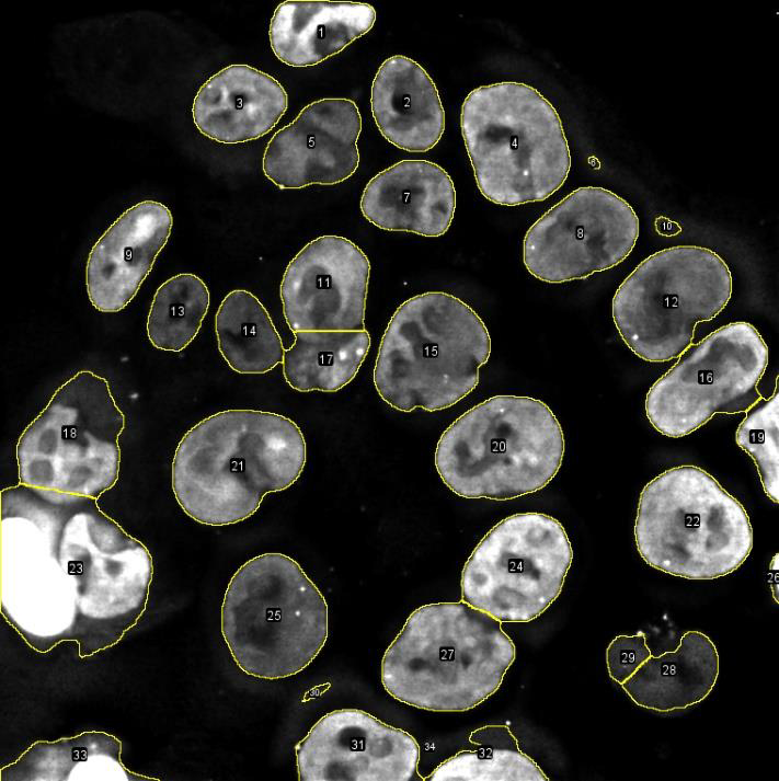
Sometimes one needs to detect bright spots that are not very bright, in a low SNR image, with a lot of unspecific signal:

In the image above, we observe a rather strong non-specific signal in the whole nuclei. The intensity of this non-specific signal versus the background is close to the intensity of the spot signal versus the non-specific signal. Even the nucleus in the image does not look happy about it.
The non-specific signal generates clear and sharp edges at the border of the nucleus, which is picked-up by the LoG detector, with unfortunately a high quality. Our goal is to come up with a better detector, with a better edge response elimination. After some tests I came up with a detector based on the determinant of the Hessian matrix.
The Hessian matrix of an image is a tensor made of the combinations of the 2nd derivatives of the intensity in all directions at each pixel of the source image. So, if f is the intensity, we have at each pixel:

(Note that it is a real, symmetric matrix.) This matrix measures the ‘local curvature’ of the intensity. In a hand-waving explanation, let’s suppose we work in 2D and that the intensity is actually the height of a surface. And let’s consider the height variation in only the 2 principal directions, that we suppose are aligned with the X and Y axes. A bright spot in the source image corresponds to a sharp peak in our surface analogy. At the top of this peak, the curvature is high in absolute value along X and negative: the height increases a lot then decreases immediately after the peak. So, the curvature hxx has a large absolute value. The same along the Y direction.
Let’s suppose now we compute the curvature not on a peak, but on a bright line aligned with the Y axis. In this case the curvature is still high along the X axis: When we cross the line, the height increases and decreases immediately. But along the Y axis, the as we follow the line, the height does not change and the curvature is 0. If we have an edge along the Y axis instead of a line, the situation is the same: the curvature is high when we cross the edge along X, but 0 along Y.
If we now extend our analogy to a surface mapped in 3D, we still have peaks and lines in 3D, but also have planes and plateaus. Let’s suppose we have a plane aligned with YZ. In this case the intensity changes a lot when we cross it following the X axis, so the curvature hxx is high. As we follow the plane along Y and X, the curvatures hyy and hzz are 0. The same for a plateau aligned with YZ.
In summary, in 3D, if we consider the absolute values of the 3 variables hxx, hyy and hzz:
- The 3 values are high in absolute value for a bright peak.
- Two of them are small for a plane or plateau.
- One of them is small for a line or an edge.
- In a homogeneous region of the image, all of them are small.
We can therefore build a spot detector that exploit this fact by taking the product of the 3 curvatures. The product will be comparatively higher only for locations at which we have a bright spot, and should offer a much lower value for plateaus and edges. The analogy above works if the principal directions are aligned with the X, Y and Z axes. When they are not, we can diagonalize the Hessian matrix (we can, it is real and symmetric) and use the eigenvalues instead. But since we are computing the product of the eigenvalues, we can take the determinant of the matrix and skip the diagonalization step to be faster.
The new detector is based on this calculation:
https://github.com/fiji/TrackMate/blob/hessian-detector/src/main/java/fiji/plugin/trackmate/detection/HessianDetector.java#L146-L228
This idea is absolutely not new. Lindeberg [1] already proposed it in the 90s along the LoG detector we have been using so far. I merely extended it to 3D. Mikolajczyk and Schmidt [2] noted that the determinant of the Hessian has indeed a stronger specificity to blobs in images with many spurious structures. Also, if this new detector is based on the product of the eigenvalues (determinant of H), the LoG detector is based on the sum of the eigenvalues (trace of H).
B. In TrackMate.
TrackMate will show a new detector with a specific configuration panel:


Spot size in XY and Z.
This detector allows configuring a different size of spots in XY and Z, to account or the elongation along Z.
Normalizing the quality value.
Also, there is a checkbox that normalizes all the pixel values of the Hessian determinant image between 0 and 1 for each time-point separately. With this checked, the spot with the highest quality will have a quality of 1. (It is possible that it gets a lower quality if you use a complex region of interest where a bright spot would be in the bounding box of the ROI, but outside the ROI.)
This will help dealing with the high bleaching we observe. Indeed, here is an example of a movie where we have bleaching. If we look at the mean intensity over time, we get this:

The mean intensity is divided by 5 from start to end, so if set a threshold on quality based on the first time-point, it is likely that we will miss relevant spots at later time-points. Inversely, if we set a threshold based on later time-point, we will have many spurious spots in the first time-points that will complicate tracking later on. If you select the ‘normalize’ option, all spots will have a quality that ranges from 0 to 1 in all time-points, which will mitigate the negative impact of bleaching.
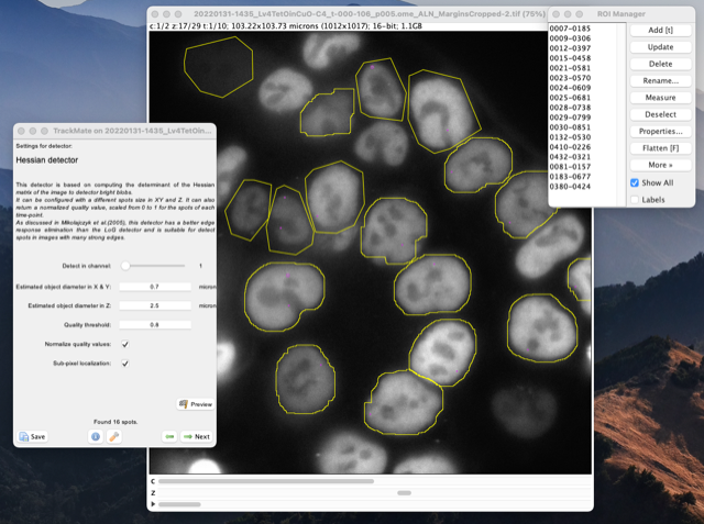
The Hessian detector can process ROIs separately.
This is super important, in particular in conjunction with the quality normalization above.
If you have the ROI manager open when you use the Hessian detector, it will treat each ROI in the list separately, and ignore part of the images that are not in a ROI.
This is incredibly useful for instance when tracking individual spots inside multiple cells in the field-of-view, as illustrated below:
Or like this:
C. Basic comparison with the LoG detector.
Now we want to check whether the Hessian detector is indeed more specific than the LoG detector. What you will see below use the parameters in the image above. I selected the Z slice in which
the spot we are tracking is present. Below you can see the results of the LoG filter (left) and the Hessian determinant (right), computed on the single cell shown above and with min & max display set from 0 to 1 and with the ‘fire’ LUT:


Both filtered images display a strong response at the spot location. However, it is clear that the LoG image has also a strong response in many other places. For instance, we observe a strong response near the edges of the nucleus. We also observe intermediate response inside the nucleus, that tends to increase local contrast this way. The Hessian image however is very specific. We only see one bright spot, and a few faint dots on the edge border. But these spurious dots are far less intense than their LoG counterpart, and they will therefore yield spots with a very low quality, making it easy to filter them out. This is confirmed by looking at the histogram of the two filtered images:


The histogram for the LoG image is very broad, while the ones from the Hessian determinant is thin. The spot quality values will be taken from the histogram, and we see that it will be easier to separate the few real spots from spurious ones on the Hessian determinant histogram. (This illustration with the histograms is inaccurate, there is not a single bin per spot, but it gives an idea.)
D. Limitations.
Also, the Hessian detector is much more demanding in terms of memory. The LoG computation can be expressed in terms of linear filtering, and uses just one convolution. To compute the Hessian matrix, we need to have the following intermediate images (in 3D):
- If the region of interest (ROI) in the source image is W x H x D pixels with 16-bit values.
- The computation of the gradients requires 3 images of size W x H x D pixels with 32-bit values (computation on floats).
- The computation of the Hessian requires one image of size W x H x D x 6 pixels with 32-bit values. The last dimension is used to store the second derivative. Because the Hessian matrix is symmetric, we only need to store the 6 elements of the upper triangular matrix.
- The determinant of the Hessian requires a storage of W x H x D pixels with 32-bit values.
The gradient image and the Hessian tensor are discarded once the determinant is calculated. But they might be large enough so that it is wide not to process several time-points in parallel. So, in this detector, the multithreading is so that each time-point is processed sequentially, and all the cores available are working on a single time-point.
Also, if you can use ROIs to delineate multiple, sparse, regions to process, you will save on computation time and RAM, compared to processing the whole image.
[1.] For a recent paper by him check Lindeberg, T. Image Matching Using Generalized Scale-Space Interest Points. J Math Imaging Vis 52, 3–36 (2015). https://doi.org/10.1007/s10851-014-0541-0
[2.] Mikolajczyk, K., Tuytelaars, T., Schmid, C. et al. A Comparison of Affine Region Detectors. Int J Comput Vision 65, 43–72 (2005). https://doi.org/10.1007/s11263-005-3848-x
An action to measure the distance from spots to ROIs bounds.

The ROIs are read from the ROI Manager. It is important that the T position of each ROI is properly defined.
This action measures the distance in XY plane. The Z coordinates is not taken into account.

After that it is just a matter of clicking the Execute button. The action computes the distance from the center of each spot to the ROI borders using the following algorithm:
- For each spot:
- Take the frame
tin which the spot belong, - Take all the ROIs that are in that frame (the T position of the ROI equals
tor0, which means that ROI is present in all frames). - For each ROI from the selection above:
- Interpolate the ROI in a list of individual points, separated by at most 1 pixel.
- Compute the distance from the spot center to the point, considering only the X & Y coordinates (the Z is not included in the computation).
- Repeat for all points of the ROI, and the min distance over all these points is returned as the distance to this ROI.
- Repeat for all ROIs, and the min distance over all ROIs is stored in the spot data.
- Take the frame
To keep the results tidy and in one place, I created a numerical feature to store this min distance. After executing the action, you will find it for instance in the tables:

And you can use it to color-code the distance to the ROI:


Export label mask spot ids.
The label exporter now has a 3rd option that allows generating a label image where each label has the ID of the spot it has been generated from (+1, not to confuse with the background with label 0).
Otherwise the labels have the IDs of the track they belong to.
'Cell shape index' morphological feature in 2D.
This introduces a new feature for spots with contour in 2D: the cell shape index
CSI = Perimeter/√Area
This is kind of redundant with the circularity, but the CSI is an adimensional variable that is used in many papers and studies in theoretical modelling.