'meanderpy' is a Python module that implements a simple numerical model of meandering, the one described by Howard & Knutson in their 1984 paper "Sufficient Conditions for River Meandering: A Simulation Approach". This is a kinematic model that is based on computing migration rate as the weighted sum of upstream curvatures; flow velocity does not enter the equation. Curvature is transformed into a 'nominal migration rate' through multiplication with a migration rate (or erodibility) constant; in the Howard & Knutson (1984) paper this is a nonlinear relationship based on field observations that suggested a complex link between curvature and migration rate. In the 'meanderpy' module we use a simple linear relationship between the nominal migration rate and curvature, as recent work using time-lapse satellite imagery suggests that high curvatures result in high migration rates (Sylvester et al., 2019).
pip install meanderpy
- numpy
- matplotlib
- scipy
- PIL
- numba
- scikit-image
- tqdm
- jupyter
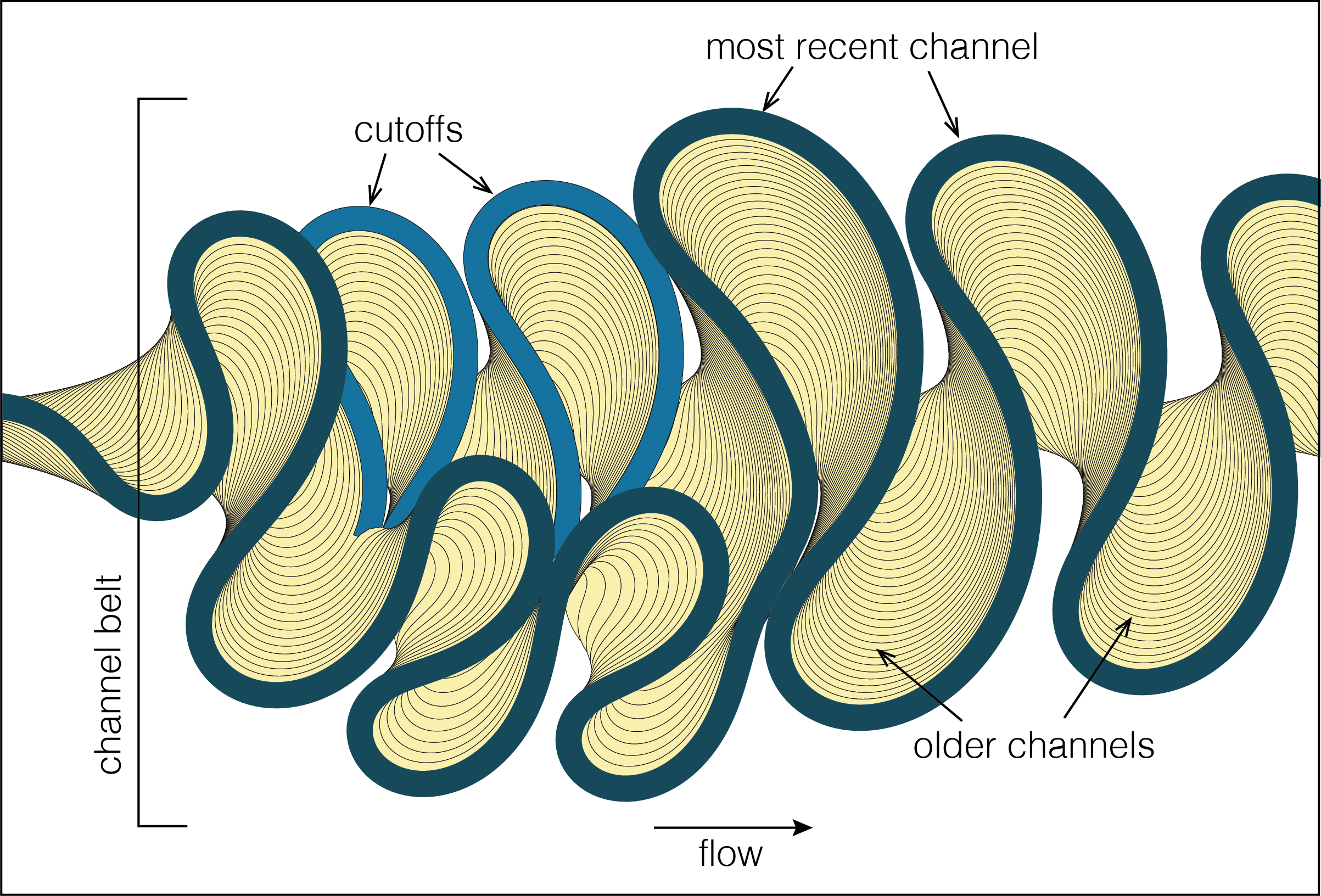
The sketch above shows the three 'meanderpy' components: channel, cutoff, channel belt. These are implemented as classes; a 'Channel' and a 'Cutoff' are defined by their width, depth, and x,y,z centerline coordinates, and a 'ChannelBelt' is a collection of channels and cutoffs. In addition, the 'ChannelBelt' object also has a 'cl_times' and a 'cutoff_times' attribute that specify the age of the channels and the cutoffs. This age is relative to the start time of the simulation (= the first channel, age = 0.0).
To run the below cells, you must first import the library:
import meanderpy as mp
import numpy as np
A reasonable set of input parameters are as follows:
nit = 1500                   # number of iterations
W = 200.0                    # channel width (m)
D = 6.0                      # channel depth (m)
depths = D * np.ones((nit,))  # channel depths for different iterations
pad = 100                    # padding (number of nodepoints along centerline)
deltas = 50.0                # sampling distance along centerline
Cfs = 0.011 * np.ones((nit,)) # dimensionless Chezy friction factor
crdist = 2 * W               # threshold distance at which cutoffs occur
kl = 60.0/(365*24*60*60.0)   # migration rate constant (m/s)
kv =  1.0e-12               # vertical slope-dependent erosion rate constant (m/s)
dt = 2*0.05*365*24*60*60.0     # time step (s)
dens = 1000                  # density of water (kg/m3)
saved_ts = 20                # which time steps will be saved
n_bends = 30                 # approximate number of bends you want to model
Sl = 0.0                     # initial slope (matters more for submarine channels than rivers)
t1 = 500                    # time step when incision starts
t2 = 700                    # time step when lateral migration starts
t3 = 1200                    # time step when aggradation starts
aggr_factor = 2e-9         # aggradation factor (m/s, about 0.18 m/year, it kicks in after t3)
The initial Channel object can be created using the 'generate_initial_channel' function. This creates a straight line, with some noise added. However, a Channel can be created (and then used as the first channel in a ChannelBelt) using any set of x,y,z,W,D variables.
ch = mp.generate_initial_channel(W, depths[0], Sl, deltas, pad, n_bends) # initialize channel
chb = mp.ChannelBelt(channels=[ch], cutoffs=[], cl_times=[0.0], cutoff_times=[]) # create channel belt object
The core functionality of 'meanderpy' is built into the 'migrate' method of the 'ChannelBelt' class. This is the function that computes migration rates and moves the channel centerline to its new position. The last Channel of a ChannelBelt can be further migrated through applying the 'migrate' method to the ChannelBelt instance.
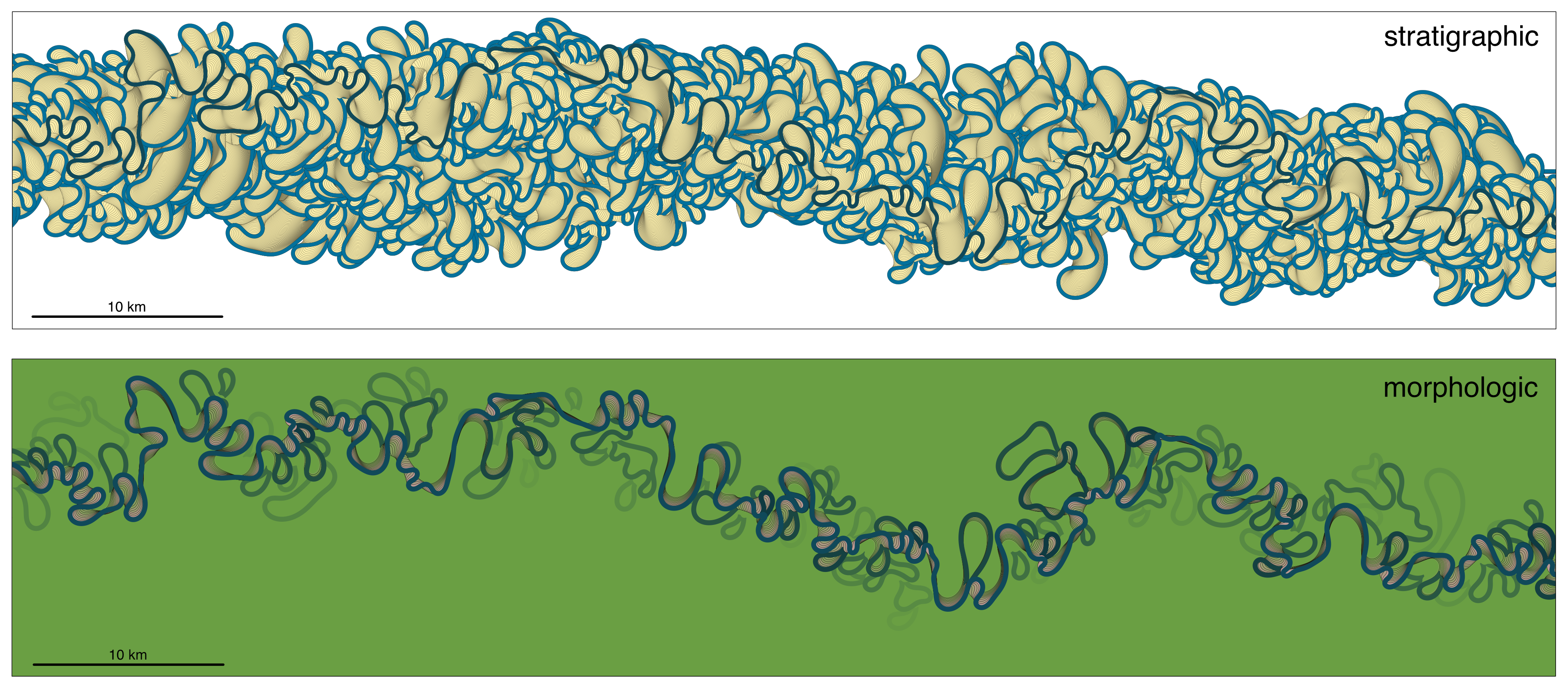
chb.migrate(nit,saved_ts,deltas,pad,crdist,depths,Cfs,kl,kv,dt,dens,t1,t2,t3,aggr_factor) # channel migrationChannelBelt objects can be visualized using the 'plot' method. This creates a map of all the channels and cutoffs in the channel belt; there are two styles of plotting: a 'stratigraphic' view and a 'morphologic' view (see below). The morphologic view tries to account for the fact that older point bars and oxbow lakes tend to be gradually covered with vegetation.
# migrate an additional 1000 iterations and plot results
chb.migrate(1000,saved_ts,deltas,pad,crdist,depths,Cfs,kl,kv,dt,dens,t1,t2,t3,aggr_factor)
fig = chb.plot('strat', 20, 60, chb.cl_times[-1], len(chb.channels)) # plotting
A series of movie frames (in PNG format) can be created using the 'create_movie' method:
chb.create_movie(xmin,xmax,plot_type,filename,dirname,pb_age,ob_age,scale,end_time)The frames have to be assembled into an animation outside of 'meanderpy'.
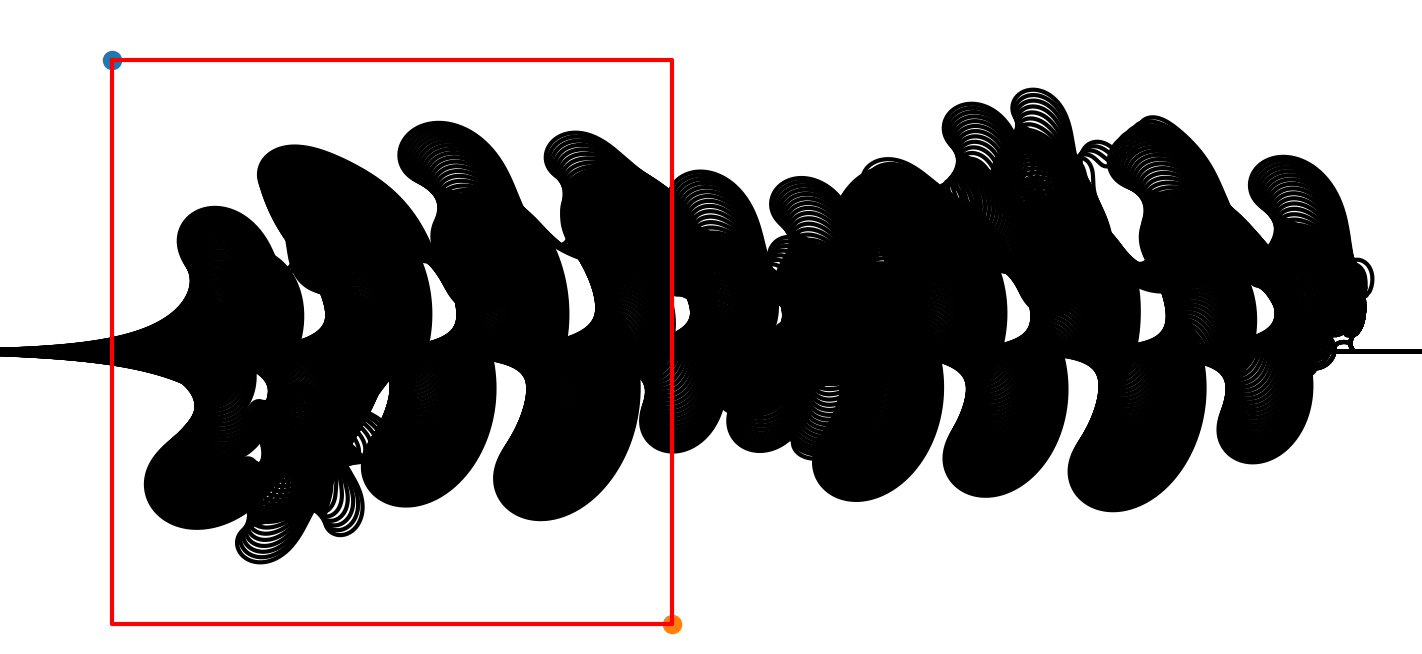
'meanderpy' includes the functionality to build 3D stratigraphic models. However, this functionality is decoupled from the centerline generation, mainly because it would be computationally expensive to generate surfaces for all centerlines, along their whole lengths. Instead, the 3D model is only created after a Channelbelt object has been generated; a model domain is defined either through specifying the xmin, xmax, ymin, ymax coordinates, or through clicking the upper left and lower right corners of the domain, using the matplotlib 'ginput' command:
Important parameters for a fluvial 3D model are the following:
Sl = 0.0              # initial slope (matters more for submarine channels than rivers)
t1 = 500              # time step when incision starts
t2 = 700              # time step when lateral migration starts
t3 = 1400             # time step when aggradation starts
aggr_factor = 4e-9    # aggradation rate (in m/s, it kicks in after t3)
h_mud = 0.4           # thickness of overbank deposit for each time step
dx = 10.0             # gridcell size in meters
The first five of these parameters have to be specified before creating the centerlines. The initial slope (Sl) in a fluvial model is best set to zero, as typical gradients in meandering rivers are very low and artifacts associated with the along-channel slope variation will be visible in the model surfaces [this is not an issue with steeper submarine channel models]. t1 is the time step when incision starts; before t1, the centerlines are given time to develop some sinuosity. At time t2, incision stops and the channel only migrates laterally until t3; this is the time when aggradation starts. The rate of incision (if Sl is set to zero) is set by the quantity 'kv x dens x 9.81 x D x dt x 0.01' (as if the slope was 0.01, but of course it is not), where kv is the vertical incision rate constant. This approach does not require a new incision rate constant. The rate of aggradation is set by 'aggr_factor x dt' (so 'aggr_factor' must be a small number, as it is measured in m/s). 'h_mud' is the maximum thickness of the overbank deposit in each time step, and 'dx' is the gridcell size in meters. 'h_mud' has to be large enough that it matches the channel aggradation rate; weird artefacts are generated otherwise.
The Jupyter notebook has two examples for building 3D models, for a fluvial and a submarine channel system. The 'plot_xsection' method can be used to create a cross section at a given x (pixel) coordinate (this is the first argument of the function). The second argument determines the colors that are used for the different facies (in this case: brown, yellow, brown RGB values). The third argument is the vertical exaggeration.
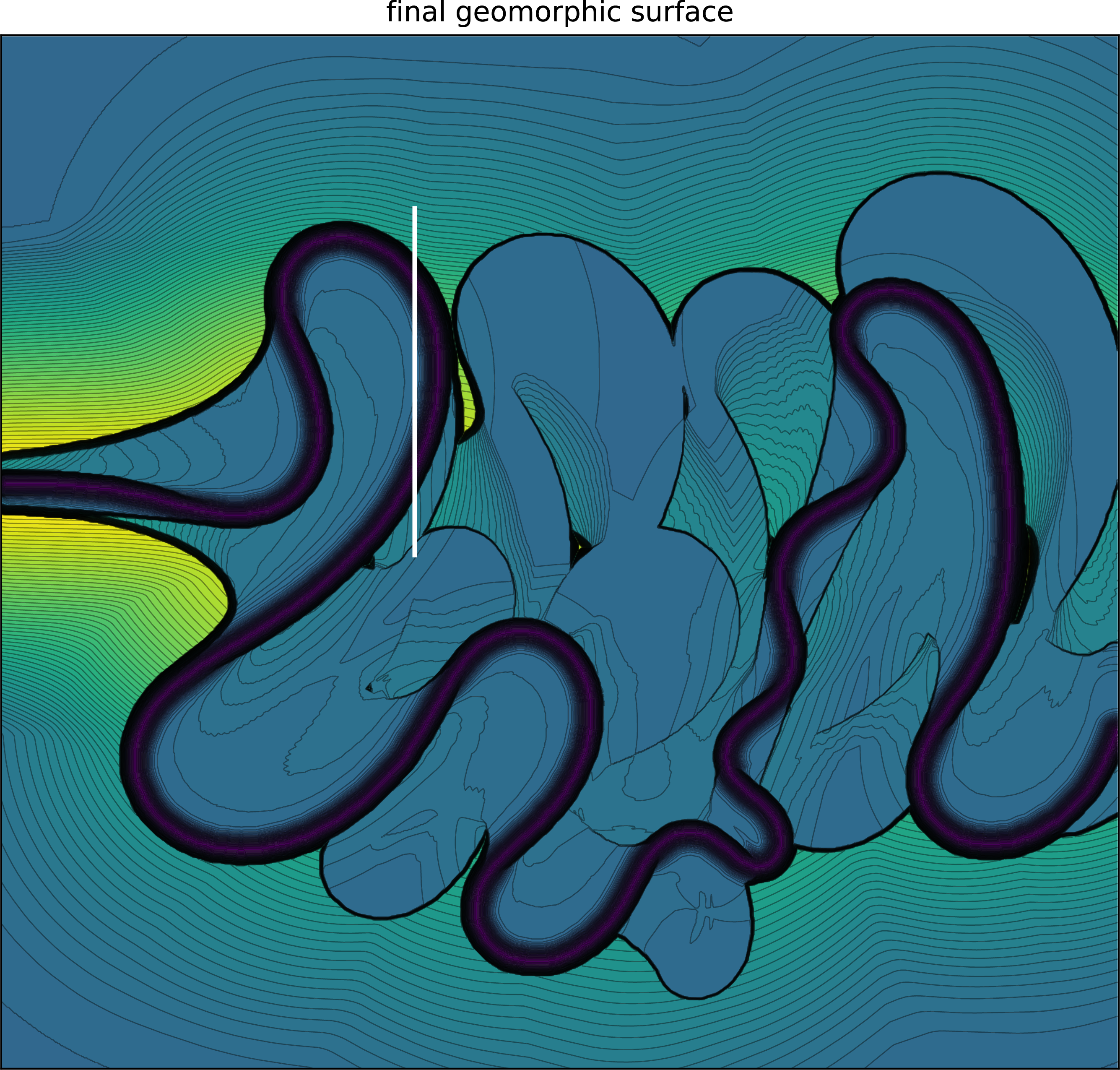
fig1,fig2,fig3 = chb_3d.plot_xsection(343, [[0.5,0.25,0],[0.9,0.9,0],[0.5,0.25,0]], 4)This function also plots the basal erosional surface and the final topographic surface. An example topographic surface and a zoomed-in cross section are shown below.
If you don't want to deal with any local Python environments and installations, you should be able to run meanderpy in this Google Colab notebook.
If you use meanderpy in your work, please consider citing one or more of these publications:
Sylvester, Z., Durkin, P., and Covault, J.A., 2019, High curvatures drive river meandering: Geology, v. 47, p. 263–266, doi:10.1130/G45608.1.
Sylvester, Z., and Covault, J.A., 2016, Development of cutoff-related knickpoints during early evolution of submarine channels: Geology, v. 44, p. 835–838, doi:10.1130/G38397.1.
Covault, J.A., Sylvester, Z., Hubbard, S.M., and Jobe, Z.R., 2016, The Stratigraphic Record of Submarine-Channel Evolution: The Sedimentary Record, v. 14, no. 3, p. 4-11, doi:10.2210/sedred.2016.3.
Sylvester, Z., Pirmez, C., and Cantelli, A., 2011, A model of submarine channel-levee evolution based on channel trajectories: Implications for stratigraphic architecture: Marine and Petroleum Geology, v. 28, p. 716–727, doi:10.1016/j.marpetgeo.2010.05.012.
While the code in 'meanderpy' was written relatively recently, many of the ideas implemented in it come from numerous discussions with Carlos Pirmez, Alessandro Cantelli, Matt Wolinsky, Nick Howes, and Jake Covault. Funding for this work comes from the Quantitative Clastics Laboratory industrial consortium at the Bureau of Economic Geology, The University of Texas at Austin.
meanderpy is licensed under the Apache License 2.0.


