AutoAnalyser

Demo to allow the user to compute transfer entropy via a GUI, and to automatically generate the code to perform the given calculation

Demos > Auto Analyser Demo

Auto Analyser Demo

This demonstration (available from release 1.3) gives you the simplest possible way to get started with an information theoretic calculation in JIDT, for measures such as mutual information, transfer entropy, etc.

The demo provides a GUI for you to:

1. select a data set,
2. select an estimator, and
3. make parameter settings for that estimator. Once you have done that, the demo:
4. Computes the transfer entropy from that data set without you needing to write any code, and
5. Generates code for you to reproduce that calculation, in each of: Java, Python and Matlab/Octave.

You have no excuses left not to use JIDT -- it is simply too easy!

This demonstration is found at demos/AutoAnalyser in the repo or full distribution.

Running the Auto Analyser GUI app

Run the AutoAnalyser GUI app via either:

1. Double-clicking your infodynamics.jar file in the top level of the distribution (note: you may need to set your OS to open jar files with Java if this is not default; and note this does not give you a console for full calculation details or errors), OR
2. Run the AutoAnalyser launcher shell script from the demos/AutoAnalyser folder, via either: a. the shell script launchAutoAnalyser.sh (may require chmod u+x), or a. the batch file launchAutoAnalyser.bat (for Windows).
3. OR to run via Matlab/Python if you do not have a separate JRE installation, open the folder demos/AutoAnalyser and run the script launchAutoAnalyser.m/launchAutoAnalyser.py (download separately if you are running release v1.5 or earlier and save in that folder).

This will start the launcher GUI app, which looks like:

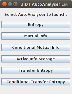
From there you can select which type of measure you wish to use, and click the button to launch its Auto Analyser, which looks like, for example:

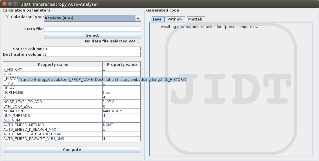
Next, you fill out the details for the information-theoretic calculation in the left panel, i.e.:

1. Select which estimator to use from the drop-down list
2. Select your data file: must be a (multivariate) time-series in a text file, with each row containing samples for each variable at the same time step, and time step increasing with the rows. The default location is our demos/data folder, which contains several sample files. If you select a Discrete estimator from the drop-down list of estimators, then make sure that you select a data file with discrete-valued data only (e.g. demos/data/2coupledBinaryColsUseK2.txt). Once you have selected a data set, the label beneath the Select button will tell you the number of rows and columns in it.
   Note: Some Mac users have reported that if the JIDT location is under Downloads, then they cannot see the demos\data files at this step (but only if running by double clicking the jar, not by running from command line). This appears to be an issue with the OS not giving file access permissions, and can be fixed by going into System Preferences -> Security -> Privacy -> Full Disk Access and then adding the Jar launcher from /System/Library/CoreServices/Jar Launcher.app as outlined here.
3. Indicate which columns of the data should be analysed (e.g. as the source and destination) for the calculation (numbered starting from 0 to match Java).
4. Provide values for all the relevant properties of this estimator in the table. The default values for each property are provided initially in the table. You only need overwrite those that you wish to change. When you hover over each property, you will see a pop-up describing the property and valid values for it (see example for property k_HISTORY in the above picture). More details are also available in the Javadocs (see Documentation) for the setProperty(String, String) method of that calculator Class. Where applicable, the GUI provides a drop-down menu (combo-box) for property value selection.

Then, click the Compute button. Unless you have made an error in the above, the information-theoretic calculation will be computed for you, and the result written below the Compute button.

Furthermore, the app will generate code to repeat this calculation using JIDT for you, in each of Java, Python and Matlab. The code is shown in the right panel; for example, see:

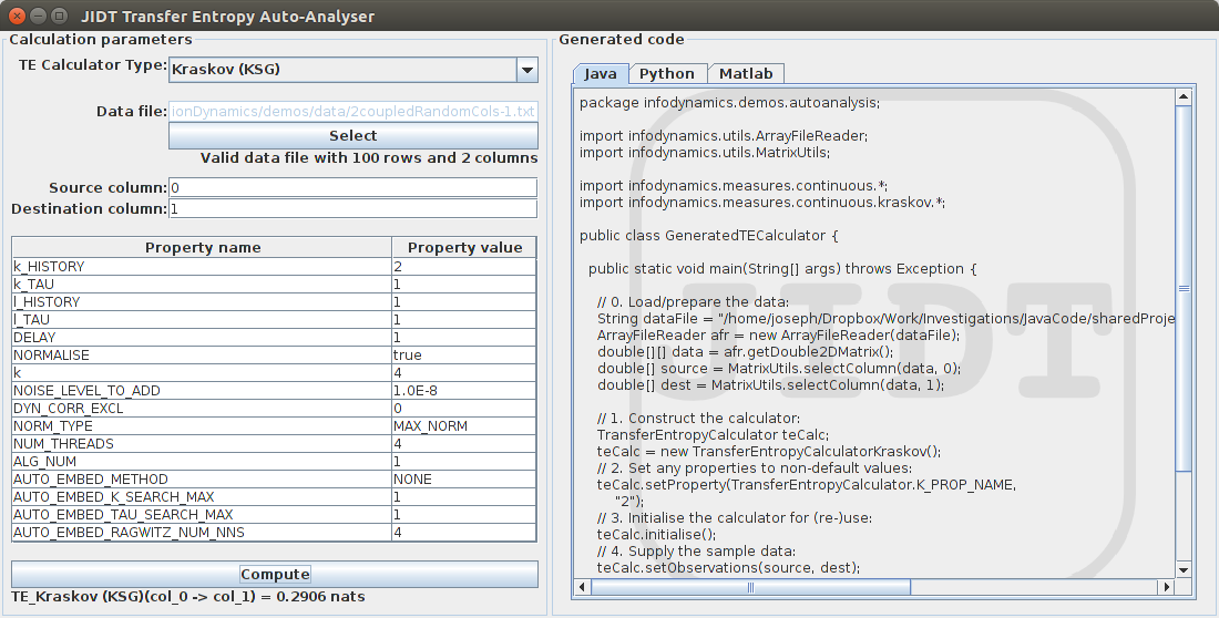
As you can see, there are separate tabs displaying code generated in each of Java, Python and Matlab.

Running the generated code files

Generated code files are also saved for you in the location of the app (demos/AutoAnalyser) for Python and Matlab, and under demos/java/infodynamics/demos/autoanalysis for Java. You can run the generated code in each language from the demos/AutoAnalyser folder as follows:

1. Java: on the command line in this folder, run .\runAutoGenerated.sh (after chmod u+x) or runAutoGenerated.bat
2. Python: on the command line in this folder, run python GeneratedTECalculator.py
3. Matlab/Octave: start Matlab/Octave in this folder and run GeneratedTECalculator You can confirm that the same result is provided by the GUI and from each of these generated programs. (Potentially small fluctuations occur when using the KSG estimator due to the addition of smal amounts of noise to the data.)

Using the GUI app to learn JIDT

A useful exercise to undertake when learning JIDT is to play around with the estimators and property values. Observe and try to understand the changes these selections make to the code that is generated. One thing you should notice is that property settings are only generated in the code where they are different to the default property values.