A Python/MATLAB reference implementation of a computationally efficient method for computing the constant-Q transform (CQT) of a time-domain signal.
Note: I just translate the core original MATLAB codes (/MATLAB/*.m) to Python version (/CQT.py) with following functions:
-
Core:
cqticqtgenCQTkernelgetCQTcell2sparsesparse2cellplotCQT
-
Extra bonus:
bufferupsampleround_half_upnextpow2hann
See the authors' homepage for more information and MATLAB packaged downloads:
Or you can read my blog post (Chinese) for inspriation:
C. Schörkhuber and A. Klapuri, “Constant-Q transform toolbox for music processing,” in Proceedings of the 7th Sound and Music Computing Conference, Barcelona, Spain, 2010. PDF or Constant-Q_transform_toolbox_for_music_processing.pdf
- Python 3.6+
- Numpy
- Scipy
- Matplotlib
Note: It might not be as efficient than the original MATLAB version, partly because the sparse property have yet to be fully utilised in this Python version.
from CQT import *
fname = './demo.dat'
data = np.loadtxt(fname)
t, hp, hc = data[:,0], data[:,1], data[:,2]

fs = 1/(t[1]-t[0])
print('fs =', fs)

bins_per_octave = 24
fmax = 400
fmin = 20

Xcqt = cqt(hp, fmin, fmax, bins_per_octave, fs,)
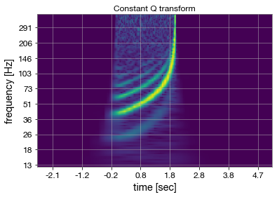
_ = plotCQT(Xcqt, fs, 0.6)

y = icqt(Xcqt)MIT
